Lognormal and power law distributions

Where does a log-normal distribution “come from”?

The log-normal distribution shows up all over the place because it arises from a quite general process. That process is the multiplication of many positive random variables. The same way we associate the normal distribution with the addition of many random variables due to the central-limit theorem, we can also think of analogous behavior in the log domain. That is if we have some random variables $X_i$ with some mean and finite variance, then the sum of all of these variables tends to a normal distribution $\sum_i X_i \sim \mathcal{N}(\mu,\sigma)$ . Likewise then, the product of many random variables $Y_i$ , is $\prod_i Y_i$ , and taking the logarithm of this expression leaves $\log(\prod_i Y_i) = \sum_i \log Y_i$ and thus the logarithm of $Y_i$ can be seen to be normally distributed.

Why is it like a power law?

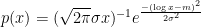
The utility/prevalence of the log-normal distribution rises too because we can see that in some approximations, it maps to a`power-law’ distribution. First writing out the precise form, the log-normal distribution function in terms of the log mean $m = \langle \log x \rangle$ and the log standard deviation $s^2 =\langle (\log x)^2 \rangle -\langle \log x \rangle ^2$ is

$p(x)=(\sqrt{2\pi}\sigma x)^{-1} e^{\frac{-(\log x-m)^2}{2\sigma^2}}$

taking the log of both sides we have

$\log p(x)=-\log \left(\sqrt{2\pi}\sigma\right) -\log x -\frac{1}{2\sigma^2}\left(\left(\log x\right)^2-2\mu\log x+\mu^2\right)$

$\log p(x)=-\log\left(\sqrt{2\pi}\sigma\right) +\frac{\mu^2}{2\sigma^2}-\log x\left[1+\frac{1}{2}\left(\frac{\log x}{\sigma}\right)^2+\frac{\mu}{\sigma^2}\right]$

but if $\sigma$ is an appreciable amount of the range of $x$ we are investigating, than the second term in the brackets is very small. Defining $b=-\ln\left(\sqrt{2\pi}\sigma\right) +\mu^2/2\sigma^2$ and $m=1+\mu/\sigma^2$ we then can re-exponentiate

$p(x)\sim e^{b-m \ln x}$

$p(x)\sim e^{b}x^{-m}$ .

Thus the probability depends on a power-law of the independent variable.

The distribution is nice because it looks linear on a log-log scale. That is if we have some distribution $p(x)=ax^{-\alpha}$ , and we take the log of both sides and plot the log-transformed variables, say $\log y= \log(ax^{-\alpha}) = \log(a) + -\alpha \log x$ , we can write this as $\bar{y} = \bar{a} + -\alpha \bar{x}$ we have a linear function in $\bar{x},\bar{y}$ space.

Notes/caution on power law distributions

I met an sociologist the other day who was studying the social networks involved in HIV epidemiology. I asked him a dumb physicist question, “what do the networks look like? are they power-law distributed?”. He smiled. “If you are used to looking for power-law distributions, then yes.”

His point was really well taken. In this example what I was asking about is the distribution of degree sizes (or number of edges coming out from nodes in a social network, or graph). That is, how many people have 3 contacts?, how many 5?, how many 50? It seems that many human networks (the internet is a good example) have multiple scales (5-50-500 etc), and that actually those distributions look linear on a log-log scale as described above. However, it has become fashionable to point to these relationships and draw out power laws. It turns out this fitting process is actually slippery, and Clauset, Shalizi, and Newman (arxiv) have a really nice albeit snarky paper on how to do this correctly, or not.

Lognormal and power law distributions

Where does a log-normal distribution “come from”?

Why is it like a power law?

Notes/caution on power law distributions

Published by dbrvs

Leave a Reply Cancel reply

Where does a log-normal distribution “come from”?

Why is it like a power law?

Notes/caution on power law distributions

Share this:

Like this:

Related

Published by dbrvs

Leave a Reply Cancel reply