
Mostly for me, I am writing a little history of mathematical models. A timeline really.
1202, Fibonacci tried to model rabbits with the eponymous sequence.
1780, Malthus tries to model human populations as a deterministic birth death process, not valid as time goes to infinity of course, but he has

where 
1820, Verhulst makes this more realistic by adding a carrying capacity that depends on resources. Thus he uses

so that 

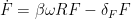
1925, Lotka writes his famous differential equations to describe predator-prey dynamical systems (1926 Volterra independently publishes… allegedly). Here I write them in terms of rabbits 


1936ish, Kolmogorov generalizes these equations
1927, Kermack and McKendrick write the famous SIR model, describing an epidemic process in susceptible, infected and recovered individuals. Typically this model is a fractional model using 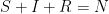


von Foerster
Zipf’s law
