Intra-host HIV model with latency

The canonical model

I end up doing calculations related to this model quite a bit, so I’m leaving it here for myself and others.

I’ll begin with what I refer to as the “canonical model of HIV dynamics”. This is an ordinary differential equation set that governs susceptible cells $S$ , infected cells $I$ , and viruses $V$ . The first prominent paper to use the model is probably the Nature paper of Perelson et al. from 1996, but more mathematical results were shown previously. I like “Dynamics of HIV infection of CD4+ T cells” by Perelson, Kirschner, and deBoer from 1993.

So, the equation set is typically written

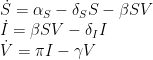
$\dot{S} = \alpha_S - \delta_S S - \beta S V \\ \dot{ I} = \beta S V - \delta_I I\\ \dot{ V}= \pi I - \gamma V$

in which the over-dot notation indicates time derivatives (e.g. $\dot{x} = \partial x/\partial t$ ). I have taken some liberties to make notation more to my preference. For example, the state variables are consistently latin, and the transition rates are consistenly greek with subscripts to denote their respective state variable. Note it doesn’t matter except for the dimensions of the rates, but typically the states are kept in units of concentration (usually per microliter). Virus is often expressed as viral load in the blood which takes viral RNA copies per mL, so we can convert that later if we like.

So, we have the constant birth rate $\alpha_S$ [cells/ $\mu$ L-day] and concentration-dependent death rate $\delta_S$ [1/day] of susceptible cells, the infection rate $\beta$ [ $\mu$ L/virion-day], the death rate of infected cells $\delta_I$ [1/day], the rate at which virions arise from infected cells $\pi$ [virions/cells-day] (reflecting an average of both leakage of virus from living cells and burst production upon cell death), and the viral clearance rate $\gamma$ [1/day].

A lot of HIV cure research these days is focused on removing “latent” HIV. This is a state where HIV has integrated its DNA into a cell, but the cell is not producing virus, thus the immune system (or medicine, more on that in a bit) does not see the virus, and doesn’t remove it. We are going to model the latent state too.

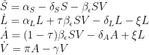
We expand the infected compartment of the canonical model to account for the latently infected cells $L$ and actively replicating, infected cells $A$ . The probability of entering the latent compartment given an infection we call $latent \tau$, and the complementary probability of entering the active compartment is $1-\tau$ .

We also separate out the dynamics because evidence shows latently infected cells live like uninfected cells, dividing to make daughter cells and dying naturally—also note there will be cool dynamics because these cells are in fact CD4+ T cells which are immune system cells in themselves and likely clonally expand to fight other pathogens… but we ignore that for now. We let latent cells proliferate and die with rates $\alpha_L$ and $\delta_L$ [1/day] while active cells die with rate $\delta_A$ . The proliferation of active cells is likely negligible relative to the fast death rate. Latently infected cells transition to active cells at rate $\xi$ [1/day]. The mechanism for this is not fully understood.

At this point too we include HIV medicine. Antiretroviral therapy as it is called is incredibly effective at stopping viral replication to the point that modern ART allows HIV-infected patients to have undetectable viral levels, and live a normal life. Still, motivation for “cure” persists because if a patient cannot take the medicine strictly, like for example if they live in a place where it is hard to get, a latent cell can reactivate and restart the infection. In the model, we denote the effectiveness of ART therapy $\epsilon \in [0,1]$ such that it can range from perfectly effective to no effect in the sense that infectivity on ART can be expressed $\beta_\epsilon=(1-\epsilon)\beta$ .

Our new set of equations is then
$\dot{ S} = \alpha_S -\delta_S S - \beta_\epsilon S V \\ \dot{ L} = \alpha_L L + \tau\beta_\epsilon S V - \delta_L L - \xi L\\ \dot{ A} = (1-\tau)\beta_\epsilon S V - \delta_A A + \xi L\\ \dot{ V} = \pi A - \gamma V$

Equilibrium solutions of the model

Equilibrium solutions to the set of ODEs above can be calculated by setting all the time derivatives to zero. We denote the equilibrium state with an asterisk).

First we solve the fourth equation for $A^*$ and multiply by $\delta_A$

$\delta_A A^* = \frac{\delta_A \gamma V^*}{\pi}$

then identify $\delta_A A^*$ from the third equation to get

$\frac{\delta_A \gamma V^*}{\pi} = (1-\tau)\beta_\epsilon S^* V^* + \xi L^*$

then solving the second equation for $L^*$ leads to

$\frac{\delta_A \gamma V^*}{\pi} = (1-\tau)\beta_\epsilon S^* V^* + \xi\frac{\tau\beta_\epsilon S^*V^*}{-\theta_L}$

so that we can factor and cancel $V^*$

$\frac{\delta_A \gamma}{\pi} = \left[\frac{-\xi\tau}{\theta_L}+(1-\tau)\right]\beta_\epsilon S^*$

and rewrite the bracketed term as 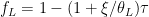$f_L=1-(1+\xi/\theta_L)\tau$ for notational simplicity and because this is all the rates related to latency. We now solve for the equilibrium value of the susceptible cells

$S^* = \frac{\gamma\delta_A}{\beta_\epsilon \pi f_L}.$

From here, we solve for the equilibrium viral load concentration, or the viral set-point using the first equation

$V^* = \frac{\alpha_S}{\beta_\epsilon S^*} - \frac{\delta_S}{\beta_\epsilon}$

and the others follow, leading to the set of equilibrium solutions:

$S^* = \frac{\gamma\delta_A}{\beta_\epsilon \pi f_L} \\ L^* = \frac{\tau}{\theta_L}\left[\frac{\gamma\delta_S\delta_A}{\beta_\epsilon \pi f_L}-\alpha_S\right]\\ A^* = \frac{\alpha_S f_L}{\delta_A} - \frac{\gamma\delta_S}{\beta_\epsilon \pi}\\ V^* = \frac{\alpha_S\pi f_L}{\gamma\delta_A}- \frac{\delta_S}{\beta_\epsilon}$

1 Comment

Pingback: Extinction in an HIV model – Daniel B Reeves

Intra-host HIV model with latency

The canonical model

Equilibrium solutions of the model

Published by dbrvs

1 Comment

Leave a Reply Cancel reply

The canonical model

Equilibrium solutions of the model

Share this:

Like this:

Related

Published by dbrvs

1 Comment

Leave a Reply Cancel reply