Beyond white: simulating colored noise in stochastic differential equtions

In physics, and elsewhere, stochastic processes are often simulated as white-noise processes. These processes are idealized and typically justified as the limit of exponentially correlated colored noise. The white approximation is not always accurate, and sometimes it is necessary to simulated colored noise.

Following Fox’s work [1], I wrote this note to demonstrate how to simulate colored noise.

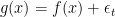
Consider the stochastic differential equation where the time derivative of state variable $x$ is given by some nonlinear process $f(x)$ as well as Gaussian white noise $\lambda_t$ . Gaussian white noise is defined by the derivative of Brownian motion (Brownian motion is called the Wiener process in some mathematical literature) $W_t$ such that

$\mathrm{d}W_t = \lambda_t \, \mathrm{d}t$

We can write a stochastic differential equation (SDE) then

$\dot{x} = f(x) + \sqrt{2D} \,\lambda_t$

where the mean of the noise is zero, and autocorrelation (correlation with itself over time) is given by the Dirac delta function

$\langle \lambda_t \rangle = 0$
$\langle \lambda_t \lambda_s \rangle = \delta(t-s)$

with $D$ the diffusion constant. Because the delta function has dimensions of the inverse of its argument, $\lambda_t$ has dimensions of $1/\sqrt{\mathrm{time}}$ and thus $D$ must have dimensions of $1/\mathrm{time}$ . The reason for calling this noise “white” is evident because the power spectrum, or the absolute value of the Fourier transform $\tilde{F}$ of the correlation in time is

$|\tilde{F}(\omega)|^2 = \left| \int_{-\infty}^{\infty} \delta(t-s)e^{i\omega t}\,\mathrm{d}t \right|^2 = \left| e^{i\omega s} \right|^2 = 1$

a constant for all frequencies. The process only requires the first two probability moments because it is Gaussian. We now have the stochastic difference equation

$\mathrm{d}x_t = f(x_t) \, \mathrm{d}t + \sqrt{2D}\,\mathrm{d} W_t$

and we see that because the noise is additive (and noticing $\langle W_t \rangle = 0$ ), the mean value of the solution is equal to the solution without noise, or the typical ODE. The fact that the stochastic equation corresponds with our typical intuition for integrals is due to a subtle distinction in the type of calculus chosen: the Itô calculus. I hope to write more about this soon.

To discretize the solution and compute numerically, we calculate an increment of the Wiener process (i.e. $\Delta W_t = \lambda_t \Delta t$ ). We can use the Box-Muller algorithm to generate zero mean and unit standard deviation Gaussian pseudo random numbers $\mathcal{N}(0,1)$ using 2 uniform random numbers $R_1,R_2 \in [0,1]$ as

$\mathcal{N}(0,1) = \sqrt{-2 \ln R_1} \cos(2\pi R_2)$

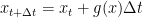
The Euler-Marayuma scheme then leads to the numerical implementation

$x_{t+\Delta t} = x_t + f(x_t)\Delta t + \sqrt{2D\Delta t}\, \mathcal{N}(0,1).$

If instead colored noise is desired, the easiest to implement is exponentially correlated noise $\epsilon_t$ defined by

$\langle \epsilon_t \rangle = 0$
$\langle \epsilon_t \epsilon_s \rangle = \frac{e^{-(t-s)/\tau}}{\tau}$

where $\tau$ is the characteristic time of the noise and $s<t$ . We computed the power spectrum of the white noise process above, and we do the same here for colored noise by taking the Fourier transform:

$\tilde{F}(\omega) = \int_{s}^{\infty} \frac{1}{\tau} e^{-(t-s)/\tau} e^{i\omega t}\,\mathrm{d}t = \frac{e^{s/\tau}}{\tau} \int_{s}^{\infty} e^{-t/\tau (1+i\omega t)}\,\mathrm{d}t = \frac{ e^{i\omega \tau}}{1+i\omega\tau}$

so that the power spectrum is for exponentially distributed noise is Lorentzian

$|\tilde{F}(\omega)|^2 = \frac{1}{1+(\omega \tau)^2}.$

We generate the trajectories of a variable $x$ experiencing exponentially correlated noise or the so-called “Ornstein-Uhlenbeck process'' by solving the system of equations

$\dot{\epsilon} = \frac{\epsilon}{\tau} + \sqrt{2D} \,\lambda_t$
$\dot{x} = f(x) + \epsilon_t.$

A subtle note is that the initial value of the exponential noise can be chosen as a Gaussian random variable so that really we have that the mean of the auto-correlation function is exponentially distributed for all initial values of $\epsilon(0)=\epsilon_0$ . So a full solver of the set of equations above is to generate $\epsilon_0$ as a Gaussian random number using the Box-Muller algorithm [2], then loop through the recipe:

(1) call $g(x)=f(x)+\epsilon_t$
(2) compute $x_{t+\Delta t} = x_t + g(x)\Delta t$
(3) generate another Gaussian random number $\mathcal{N}(0,1)$ with Box-Muller and two new uniform numbers $R_3,R_4$
(4) compute $\epsilon_{t+\Delta t} = \epsilon_t (1 + \frac{\Delta t}{\tau}) + \sqrt{2D\Delta t}\,\mathcal{N}(0,1)$ and return to step 1